

I almost cant believe that I am writing this blog, in truth… I had another lined up but through an accident of misaligned neurons it’s very existence has been called into question (that is… I forgot what it was about). For me this is a deep departure hence the title “Poacher Turned Gamekeeper”, any techies amongst you will of course realise that the picture above is a massive clue as to what I shall be blogging about. The image shows that infamous Easter Egg “Dev Hunter” which was of course embedded into Excel 2000, sadly a practice that rarely comes out of Redmond nowadays as they seem to have all grown up… So yes, Excel. Thats right I said Excel, which from someone who expends a great deal of energy on a weekly basis wrestling with this ‘database of choice’ it seems incredibly ill advised that I blog about it. My usual mantra is that if you want to store data about ANYTHING, then use a database and never a spreadsheet, we have an overabundance and overreliance on them in industry today and my work logs prove that! I digress…. Excel is what I’ll be covering in my blog today, only a small feature but one which saved me a (metric) tonne of time this week and I thought I’d share it with you. I have a spreadsheet which I manage on behalf of a client which captures average exchanges rate (for a given month) for a couple of currencies (US Dollars and UK Pounds) expressed in USD and EUR. This data is historical back to 2011 and is displayed within the spreadsheet in date order and then currency.
- Row 1 would be thus be January 2011 Pounds to USD and EUR
- Row 2 would be thus be January 2011 Dollars to USD and EUR
- Row 3 would be thus be February 2011 Pounds to USD and EUR
- Row 4 would be thus be February 2011 Dollars to USD and EUR
- Row 5 would be thus be March 2011 Pounds to USD and EUR
- … etc
Ignore the fact that you dont need to convert USD to USD. I know! Its just a generic capture mechanism.
This sort order makes it easy to add next months data, you just add two new rows to the end of the spreadsheet, one for GBP, one for USD; et voila….However this week I found that I need to add two new currencies for all of these dates to the spreadsheet, Indonesian Rupiah (IDR) and Saudi Riyal (SAR). I obviously didnt want to go inserting two rows, every two rows, within the spreadsheet as this would have taken forever and I would have been tempted to gouge my own eyes out with the smallest denomination of coin I could find so instead I decided to just create the new rows at the end of the document. This is all well and good for the ETL process that consumes this spreadsheet, it doesnt care about the order, it just cares about the data. Humans however need some kind of order otherwise the job just becomes harder.
- What happens next month?
- How do I copy forward the last four rows of data now?
- What if I need to change a row of data for IND in March 2013?
- How will anybody else understand this document should I fall under a bus, which btw, living in North Devon, is less likely than say …. being hit by a stray meteorite signed by the late great Charles Darwin.
What is needed is to re-sort the document properly so that mere mortals can understand it. This sample will walkthrough using the Excel Sort function (which has a nice feature I’d like to share) to sort our original GBP and USD data. The data is currently sorted by Year (Column B), then by Month (Column A) and finally by Currency (Column E) such that all of Aprils exchange rates are displayed together. What I actually want to do though is to break this data apart so that it is actually displayed by Currency\Month\Year.
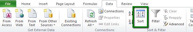
So how do we go about this, well we start by selecting all of the data and then switching to the ‘Data’ ribbon and selecting the ‘Sort’ option
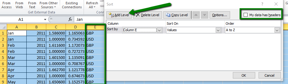
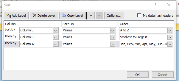
We should then see the following dialog which allows us to start setting up our sort, lets start by grouping all of the currencies together by first of all sorting ‘A to Z’ on Column E (Currency).
Now… I know what youre thinking, ‘Column E’? Thats such an ugly way of referring to this column. But you know what, Get over it… this isn’t ‘Numbers’ which takes your headers (when defined and uses them as names instead which is way more sensible!) Note that this data has no headers anyway so the point is moot, because of this the indicated checkbox remains unticked. If we did have header data we could tick this to ensure that our headers do not get sorted as well. Bygones….
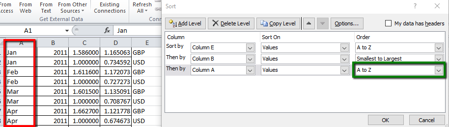
On with the show, our sort is more complex than this single field sort though and so we need to set add a few more ‘Levels’ of sort.
We thus press the button twice adding two new levels and define our secondary sort as being on Column B ( Year), because this is numerical data Excel defaults to ‘Smallest to Largest’ which is exactly what we want in this instance. For the third level we wish to sort by month but the more astute amongst you may by now be smelling Rattus Rattus; We select Column A (Month) but of course ordering using ‘A to Z’ is not at all what we want, we instead want them displayed in date order (i.e. Jan/Feb/Mar/ etc)
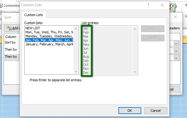
We thus need to open the ‘Order’ dropdown and select ‘Custom List’ which is that feature I wanted to share. This allows you to define your own list, or use the pregenerated sets. Luckily we have been fairly standard and so we are able to use the predefined ‘Jan,Feb.Mar…’ list.
Press ‘OK’ and you should have a screen a lot like this.
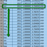
Upon pressing the ‘OK’ button again your data should be reordered as you desired. As you can see all of the GBP data is displayed together ordered by ascending date and of we scroll down you should see that in September 2017 (where my data ends) we then start to display the USD data, again all grouped together in date descending order.

Job done and I’m off to make myself feel better by shooting some pesky pheasants, that way balance can be restored….