Exploring Partitions – Reading (In Which Charles Darwin NEVER hangs out in the Cookery Section)

You know the Shtick right, you’ve got a large transactional database which month by month grows seemingly exponentially in turn leading to a severe degradation in performance. You ask the question that horrify most stakeholders “What data can we lose?” which is where somebody says… “Can we not just archive it off to another table? We don’t really need it….”. True, this deals with the immediate issue in that you’ve managed to get some responsiveness back in your main transactional table. This is all well and good up until the moment that, likely the same person who said “We don’t really need it….” realises that they do in fact need that data. In effect they’ve just pushed their performance issue into another data-table.

Don’t get me wrong, archive tables are a great tool, especially when designed into the solution from the outset, but they all suffer from the very same problem which is inherent in any large data store and that is speed.

We have a database based upon a .NET web application that we developed some years ago that deals with the thing that all companies do at the end of every single month, reconciling the data within the accounts with the real world. In principle this is very simple.

• An update is run nightly to bring on board any new/updated data
• On the first of the month one team has access to a set of frozen data, Their effort over the next few days is into signing off the end of month accounts.
• The second team in contrast can see, but cannot adjust, new/updated date. They use this data to check for issues in the feed systems
• Once the end of month accounts are signed off two things happen.
  • The signed off account data is added to an archive table, using an Archive Data to differentiate the data from previous months
  • The two streams of data (signed off and new/updates) are then re-synchronised.

This whole strategy was designed in from the start and works exceedingly well; It allows for that other thing ‘End of Year Accounting’ to be handled in a much improved manner with the Finance teams able to easily compare the accounts at points in time. That’s not to say that it could not be improved upon.

Despite being a database developer for a very long time, there are areas that I’ve never properly investigated due to time, platform or project constraints. Partitioning Data has been one of these areas; Yes time has been one element but there’s also been the fact that until SQL Server 2016 it has only been available in Enterprise SQL Server which costs many, many SATS. However as of SQL Server 2016 onwards partitioning is now available in all editions and so becomes something that is achievable for any customer. It is a big area to cover though, so I will likely cover this in a few blogs. This first blog will look a little bit at how Partitioning works and will cover query comparisons between Partitioned and Non partitioned data. The database I shall be using is relatively small with approx 6m records (though this currently) grows by 1m every 2 months.

What is Partitioning

In it’s most simple representation Table Partitioning is the database process by which large amounts of tabular data are split down into multiple smaller sub sections of data.

Splitting the table like this has many benefits:-

• Faster reads are *possible* due to the data being segmented. This is because of a methodology called “Partition Elimination” whereby vast numbers of records can be eliminated from the search due to the fact that particular Partitions contain no matching data.
• Faster writes are possible as you may elect to update only a subset of the entire dataset and ‘switch it in’ once complete
• This ‘switching in’ allows for zero down time on live database systems, even during an update process, as the data is updated ‘out of place’ (i.e. in another table) and then the lightning fast switch of the data occurs when the data is ready to be published.
• There is also the concept of ‘switching out’ whereby data can be removed entirely, or archived to a another table, instantaneously. Ordinarily this would involve a Delete of many many rows and a possible insert too which would be a lengthy process.
• Faster reads of more widely utilised data can be promoted by the hosting of most commonly queried data on faster disks, relegating rarely queried data to much slower and inexpensive drives.

Of course, as with anything that makes life simpler there are payments due, these being:-

• Complexity, Partitions are complex to set up and even more complex to maintain and alter at a later date.
• Best practices can also add another layer of complexity, and can at first seem pointless.
• Many ways to skin the same cat.
• Partitions don’t enforce, but they do *encourage* through performance losses, particular querying characteristics. If you partition a massive table by an Archive Date field and then completely fail to use that field within your where clause you will be punished.
• In order to reap the rewards of the faster update processing you will need to change your code and the way you effect an update, and it wont be simpler. It will however likely be faster and more resilient for toward allowing 24/7 uptime.
• Its not a silver bullet for poor performance. Partitioning is a strategy that can assist with a number of issues and technical requirements . It is not a plaster to cover poor design and implementations

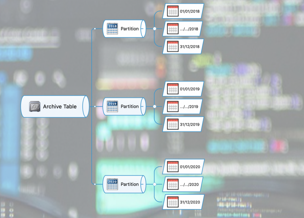
In our test we’re going to start with two identical databases, each containing an archive table with 6million rows of data. The archive tables are logically ‘partitioned’ by usage of the ArchiveDate field. That is, each dataset present within the data will be written once, and once only, into the archive table for each archive date. In our example this archive is recorded as having being recorded on the last day of each month. The first thing that should be noted is that rather unusually we have our actual dates value stored away in a dimension table. The dates (and their component parts) are stored in a table called DimCalendarDates whilst the actual archive record itself merely points to that date record using a surrogate id.

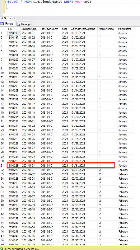
Lets take a look at the DimCalendarDate table, As you can see the actual final day within January that we are going to archive on has been circled red. If we were going to partition our table it thus makes sense to use that SID value of 2194226 as our partition value for January 2021. As you can see our SID values are incremented by one each day, this fact is important as it means that our data is consistent.

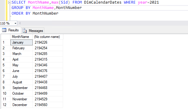
Delving a little deeper lets look at all the values from 2021 that we would want to partition by. If we look only at 2021 data, group by each month and pick the highest SID from each we will see the following data. As you can see the January value matches up with the circled value mentioned earlier. These SID values are the ID’s we would use to create our partitions

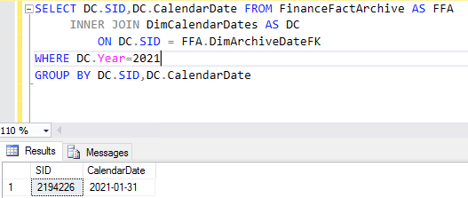
If we then bring our archive table into the equation and look for all of the archives so far created in 2021 we can see that there is only one, that is because this blog was written at the start of February and so no other archives have yet been performed. As you can see the Archive table has an Archive Date that references that January 31st date that we first spoke of with a SID of 2194226

Lets take a look at the Partition definition language now just to see what we exactly need here. Partitioning starts with a function, at least, in our case it does… You can get really complex and start at the file group level but to be honest thats far beyond this simple primer.

CREATE PARTITION FUNCTION FinanceFactArchivePartition (INT) AS RANGE RIGHT FOR VALUES (1000,2000,3000,4000)

Example Partition Function Script

So what this piece of script is saying is simple, create a partition function that accepts Integer range values as its partition key. In addition to that we are specifying the keys 1000,2000,3000,4000 as being the lower boundaries for our values? Why lower I hear you say? Well, thats what the RIGHT part of RANGE RIGHT does. If you were instead to choose RANGE LEFT those values would instead be upper boundaries. Generally RANGE RIGHT is more intuitive, and indeed in cases such as handling actual date time values is more reliable. That’s great but for us this statement really wont work as we don’t want to be dealing with hard coded values. Instead we want to obtain these partition locations from our DimCalendarDates table and use those values. I thus created this snippet of code to create all of the End of Month partitions between two dates (2017 and 2050).

/* Create the Partition Function */

DECLARE @IDS nvarchar(3800)
DECLARE @StartYear int = 2017
DECLARE @EndYear int = 2050
DECLARE @Sql nvarchar(4000)

SELECT @IDS = COALESCE(@IDS+’,’,”)  + CAST(Data.LastDayOfMonthSid as varchar) FROM (
SELECT Year,MonthName,MAX(Sid)AS LastDayOfMonthSid
FROM DimCalendarDates AS DC        
WHERE DC.Year IS NOT NULL AND DC.year BETWEEN @StartYear AND @EndYear        
GROUP BY Year,MonthNumber,MonthName) AS Data

SET @Sql = N’CREATE PARTITION FUNCTION FinanceFactArchivePartition (INT) AS RANGE RIGHT FOR VALUES (‘ + @IDS + N’)’PRINT @SQL

EXEC SP_executesql @Sql

This piece of code effectively reads all of the SIDS for the last of each month in the specified years into a comma separated variable (@IDS) and then adds this variable into a CREATE PARTITION function as we did above before executing that SQL. Once the Partition function is created we can move onto creating a Partition schema.

CREATE PARTITION SCHEME FinanceFactArchivePartitionSchema AS PARTITION FinanceFactArchivePartition ALL TO ([PRIMARY])

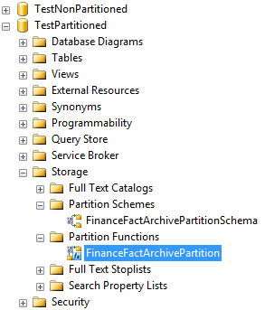
A partition scheme is necessary and effectively binds a partition function to its relevant file groups. In the above example we are binding only to the Primary file group. Once you have run these commands against your database you will be presented with something similar to this.

We now have the underlying infrastructure, so lets go ahead and apply the partition to our table. Currently we have a clustered index on our main SId column. Strictly speaking this is not required so we shall drop it and instead create a clustered index on our DimArchiveDateFK column. Note that this is not a unique column but we’re going to go with that for simplicity.

ALTER TABLE [dbo].[FinanceFactArchive] DROP CONSTRAINT [PK_FinanceFactWorkingArchive] WITH ( ONLINE = OFF )

/* Create the New Clustered Index using the Partition function to define the storage locations */

CREATE CLUSTERED INDEX IX_ArchivePartitionIndex ON FinanceFactArchive(DimArchiveDateFK) ON FinanceFactArchivePartitionSchema(DimArchiveDateFK)

After running this upgrade script, the execution of which may be quite costly, our table will be properly partitioned. The instruction is essentially saying

CREATE CLUSTERED INDEX IX_ArchivePartitionIndex ON FinanceFactArchive(DimArchiveDateFK)

Create a clustered index on the DImArchiveDateFK column

And then…

CREATE CLUSTERED INDEX ….ON FinanceFactArchivePartitionSchema(DimArchiveDateFK)

Use the DimArchiveDateFK field to bind to the FinanceFactArchivePartitionSchema Partition

So lets take a look at the data within these partitions…. We run the following piece of SQL to view our partitions.

SELECT *

FROM sys.partitions AS PINNER JOIN sys.objects AS OB    

ON OB.object_id=P.object_id

INNER JOIN sys.index_columns AS ID    

ON ID.object_id=p.object_id AND ID.index_id=P.index_id

WHERE OB.name='FinanceFactArchive'

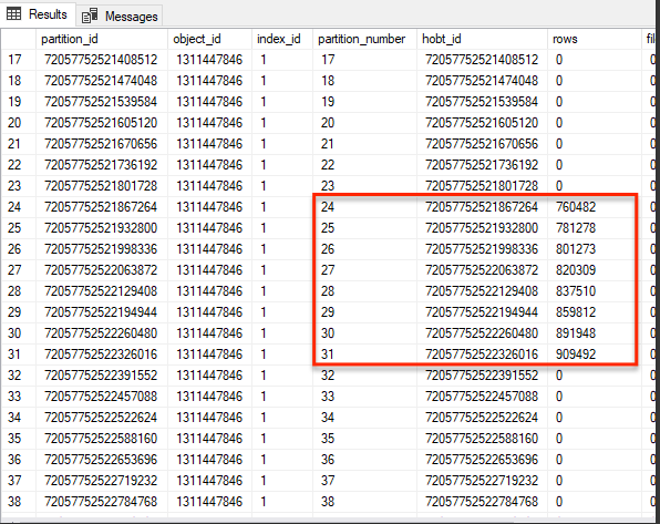
What I see within my data are a lot of empty partitions, but then again I added nearly 40 years worth of monthly partitions into a database in which I only have 8 months worth of data. However… If I scroll down the list I can see the following partitions which do contain data:-

Obviously if we look in the non partitioned database then we see no such thing, all the data is stored on the one ‘table level partition’

Cool, lets try and see how this partitioned database performs against a non partitioned database when it comes to querying. Now… There is a rule when it comes to querying partitioned data that says “You should always include the partition within your WHERE clause’…. So lets break this rules right off the bat; Remember this database is not massive… Lets try running this simple piece of SQL

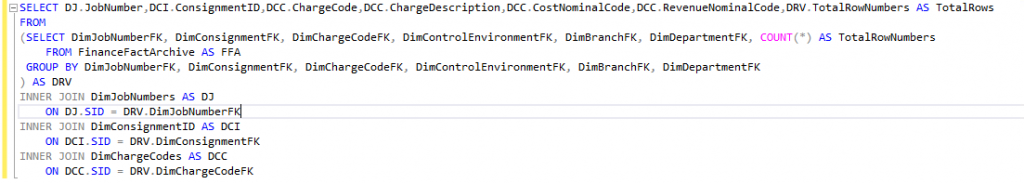
Its a bit of a nonsense query just to prove my point above and beyond a standard SELECT * statement. Upon running it against the two database we see the following performance times (this is a reasonably low spec server to further exacerbate any issues we may well see):-

Non Partitioned Date	Partitioned Data
00:56 seconds	01:11 seconds

Not a huge difference, but then again…. not a huge database and we’re actually not really performing a very complex query. Step up the complexity or the volume a little and that disparity may widen even further.

Lets step up the complexity of our query a little but abide by the partitioning rules. We’ll create a query that returns two distinct sets of archive data for two different months and then join those values to a master set of those two months worth of data. We can thus see months that have changed, months that were added and months that were deleted. The SQL which you really don’t need to understand looks like this.

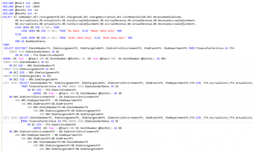
Lets have a look at the relative querying speeds of running those identical queries against identical data.

Non Partitioned Date	Partitioned Data
02:18 seconds	00:44 seconds

Thats quite a significant turnaround in the fortunes of our two database and is due entirely to the fact that the database may now omit reams of records through ‘Partition Elimination’; That is the query planning process will simply ask “What partitions are needed to return this query?” and it will ignore all others without even needing to look. In a database of 6 millions records being able to ignore the vast majority without even looking at the data is a huge boost to performance. Its a little bit like walking into any Central Library and knowing that you don’t have to look on every single shelf to find ‘On the Origin of Species’. It wont be in the children’s section, nor young adults, nor horror or cookery and not the fiction department. In fact you can eliminate most of the library shelves because the historical scientific book would never reside anywhere but in a logical place.

I refactored this query to bring a third set of data in just to make sure that it was not a one off situation, that query was slightly more complex and rolled in with the following execution times.

Non Partitioned Date	Partitioned Data
02:14 seconds	01:02 seconds

As you can see properly partitioning your database can make a huge difference to the querying times, especially in an archive database where you are dealing with metric tonnes of data (which I was not). You don’t have to lose all of your archive data and querying ability just because it has rendered your database impossible to read; A well designed partitioning schema can give you back control over your data, probably ALL of it for that matter. There has been a great deal written about partitioning by far more intelligent people than I, so if this has whetted your appetite at all I suggest that maybe a good place to start would be the rather excellent Brent Ozar and Kendra Little blogs and vlogs. They really are EVERYTHING SQL Server.